This paper is an abstract of our research that we made for the Design & Technical European Group in Arup.
We are now working on a second phase in which will be involved construction companies to test and validate the method. This study does not revolutionize the current paneling methods, but the approach is quite new.
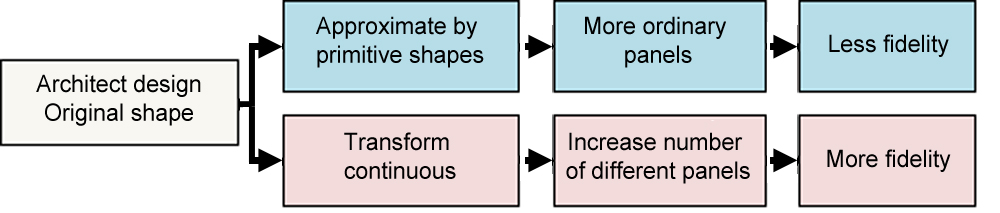
In the continuing research of complex and original architectural shapes, at certain point, in order to help the construction process and to maintain the costs on a reasonable level, we have to follow two different ways.
The first approach is the geometry rationalization, by using primitive shapes that approximate the original architecture. In this way, we can obtain a simple and ordinary paneling of the building envelope, but we can lose the fidelity compared on the original shape and we fall short on client/architect expectations.
The second approach is based on a transformation of the original continuous shape in a discrete geometry. In this way, we can obtain a paneling closer to the architectural shape, but involving in a higher number of different panels, depending on the original complexity.
By following this second way, the geometry team of the Milan office is working on a series of geometrical procedures able to optimize the number of different panels in a free form surface, by using Rhino and Grasshopper.

Objective

The objective of this study is to define a tool in Grasshopper/Rhino which allows creating and manipulating on a free form surface (input) different type of paneling (output).
The criteria are:
• Study a geometrical approach able to define a serial paneling.
• With this tool we work only on the size, position and shape for each panels.
• We don’t change the original shape.
The first criterion is to reduce the number of different panels and optimize the final result. This tool allows managing the position, orientation and size of the panels on the surface.
The second criterion is to allow controlling the gap between the panels. In this way we want to reduce the number of different panels and adjust the panels positioning on the construction phase, by managing the gap.

Observation

In nature there are many examples of tiling, and by the evolutionary process nature use “geometrical tricks” to achieve the best solution. The objective is to minimize the energy consumption in the life process (less and simple instruction = lower energy consumption). An example of tiling in nature is the pattern of the crocodile skin. There are similar examples in the natural environment, like in the landscape erosion process or in the crystal geometrical creation process.

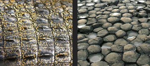
Image 1-2: On the left crocodile skin (quadrangular pattern); on the right “Giant's Causeway, Ireland” (hexagonal pattern).

Although the difference between natural world and cladding of complex building are clear and obvious, the way we want to follow is similar. In the contemporary architecture, there are many examples of buildings with complex surface cladding made with different approaches: one way is to use different panels that perfectly follow the shape. The problems with this solution are the major cost of providing a big amount panels all different, and during the life cycle, the maintenance and panel replacement.

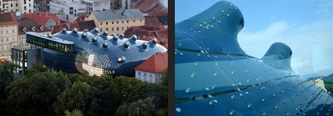
Image 3-4: Bix-Kunsthaus, Graz, Peter Cook and Colin Fournier. Cladding with double curvature panels. The panels are all different.

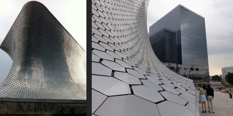
Image 5-6: Museum Soumaya, Mexico City, Fernando Romero. Cladding of hexagonal pattern. The panels are all different.

Another approach is to cover the surface of the envelope by using modular elements: equal panels that include some type of connection joints to the building. This kind of cladding partially covers the surface, and the trick to cover the shape is varying the gap between the elements. In this kind of envelope the construction cost is lower (depending on materials, panel’s size, etc.) and the maintenance during the building life cycle is cheaper and easier

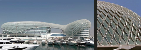
Image 7-8: The Yas Hotel, Abu Dhabi, Asymptote Architecture’s. Cladding with variable gap between elements.

Images 9-10: Selfridges department store, Birmingham UK, Future Systems. Also on this example the cladding elements are equal, but the gap changes.

Only paneling of flat and single curved surfaces can be obtained by a single panel type. For geometries with double curvature, like spheres, torus, or free form shapes, must be provided a tiling with a series of different panels. For primitives geometries (sphere, torus, cone) it is possible to optimize the result by minimizing the number of panels, depending on the size of the panels. The free form sheet, compared with the other type of geometries shown, is evidently the worst case.

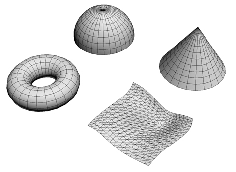
Image 11 – Some examples of double / multiple curvature surfaces: hemisphere, cone, torus and free form sheet.

The free form surfaces is the object of our studies. The first tool called the “analysis tool” used to compare different solutions.

Analysis Tool

To compare the different solutions we need an automatic tool, that produces the result quickly and easily.
The analysis tool can produce these outputs:
• Number of panels.
• Number of panels families.
• Space distribution of equal panels.
• Frequency of panel’s types.
• Frequency of equal panels edge lengths.
• Variety of panel edge length.
The tool colors a facetted façade with a gradient following the same pattern of the spectrum according to the perimeter of each panel. The smallest panels will be colored in red while the biggest will be in violet, through yellow, cyan and blue. Equal panels or very similar ones will have the same color. In order to add more flexibility, the analysis script has an added parameter: the tolerance within which two panels can be considered the same.
According to the tolerance parameter it is possible to understand how adding or removing the gap between panels affects the global repetition of the façade.
The analysis tool will be useful for understanding the effectiveness for each method of rationalization showed in this document.
This tool is also useful for the analysis on tiling modeled with any method or software; so it is a versatile tool. It is sufficient insert as input a series of triangles. Sometime the triangles are obtained cutting surface of different shape, in this case you can use the “rebuild cut surface” module.

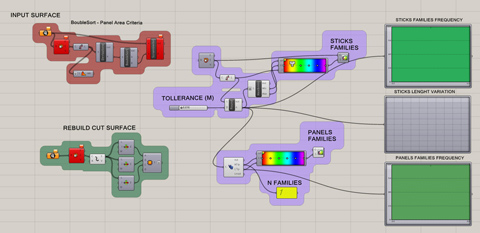
Image 12 – Tool scheme(Grasshopper)

The method

This chapter discusses the process adopted to define the paneling tool. For this purpose we have been using various software’s. Not all exercises have led to satisfactory results, but the proceedings were still useful to understand the right way to follow.
The major activities are:
• Simulation by dynamic solver
• Definition of a UV grid on a Nurbs surface
• UV distribution of equidistant points on a Nurbs surface
• Hexagonal pattern of a grid points that starts from origin.

Simulation by dynamic solver

The first idea was to compare the tiling of a building envelope to the behavior of a group of coins which stay by gravity on a surface. The question is: How can a group of coins be conforming to a surface to obtain the minimum distance among each other?
Obviously, the best distribution of a group of coins (the same type of coin) is on hexagonal pattern. By using only coins with the same size, all the coins have six tangency points (honeycomb pattern).
The process starts from a group of cylindrical meshes that simulate the coins. The cylinders are connected by 3d-rotational constraints on the tangency points; each coin has six tangency points/constraints with the adjacent coins. The final result is a planar grid oriented on the XY plane, including all the coins in the simulation.
The next series of images (image 13) show four steps of the process: the group of coins starts from a fixed position close to the curved surface (A), the dynamic solver starts and calculates the falling by gravity (-Z vector). The falling simulation is not 100% correct, not all the constraints work properly and some coins move out the grid position (B and C). In any case, in the final image of the sequence (D), the collision with the double curved surface reflects quite well the reality: most of the coins are conformed to the surface, only few coins don’t touch completely the surface.

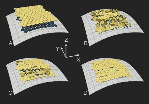
Image 13: four steps of the animated sequence of the falling coins.

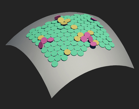
Image 14: simulation that shows the different coins behavior.

Image 14 shows the coins by colors that represent different behavior: green – the coins perfectly touch the curved surface; yellow – the coins are moved on different direction; red- the coins move more than the yellow. By this test we learn the following considerations:
• A group of coins connected by hexagonal pattern grid cannot completely conform to a double curved surface.
• Depending on surface curvature and coin size, most of the coins conforms the surface (like the greens in the simulations previously described); there are only few yellow and red coins.
• This means that is possible to cover a free form envelope by only one type of cladding panel, except for some local areas were we need to provide special panels, with proper size and shape

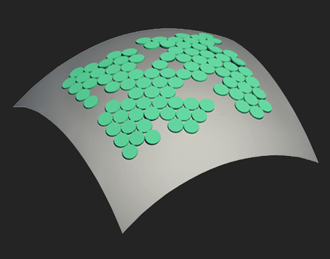
Image 15: hexagonal pattern of circle. The green circle can have different radius, depending on the curvature of the conforming surface.

Definition of a UV grid on a Nurbs surface

One of the most used methods of tiling is subdividing a surface following UV coordinates.
In the common modeling software the surfaces are made by a wire of Non-Uniform Rational B-Spline (NURBS) curves.
There are two types of curves, U and V: U curves follow a direction while V curves are perpendicular or pseudo-perpendicular direction like the rows and columns in a table. They make a mesh and for each intersection there is a control point. This is a sort of coordinate system that can define and describe any complex surface.
The simples subdivision method is using directly the same definition of Nurbs mesh or rebuilding a new mesh with an interpolation using more or less curves in V or U direction. So this type of tiling is a regression of polynomial curves into a series of segments. Although this timing method doesn’t pay any particular attention to the serialization issue, it is certainly the way that approximates better the starting geometry. The panels that are obtained by this kind of subdivision usually change dimension in a gradual way, practically they are all different and they have, between the smaller and the bigger, important dimensional variations.
This method is the easiest, but it is not recommended. In the construction phase you may have a lot of technical difficulties related to the great number of panel types and to the great geometric variability between smallest and biggest elements.
However the panels obtained with this method must be not cut on the façade border, so this tiling is better on the peripheral of global surface. In the event that you have to work on very small surfaces, with few panels or very twisted or complex surfaces, with a lot of parts also convex or too concave, often the UV coordinates subdivision is the only possible way.

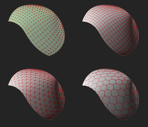
Image 16: Different UV subdivisions on the same surface

Distribution of equidistant points

An interesting method of subdivision of the surfaces in the panel is to operate through the creation of a mesh of points equidistant from each other lying on the surface itself. You can create a grid of skew quadrilaterals with all sides equal and diagonal dissimilar.

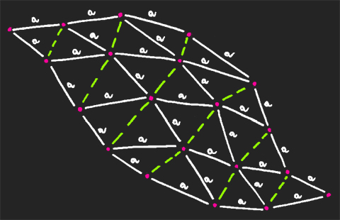
Image 17 - Equidistant Points Distribution

In order to obtain this type of subdivision is necessary to define a point on the surface and then proceed to expanding rings for definition of other points.
Is this necessary to draw the locus of equidistant points from the starting point to a predetermined distance; this locus is similar to the loci that define the circumferences on the floors, hereafter we will call it pseudo-circumference and it can also be seen as the intersection between a sphere of radius equal to the predetermined distance centered on the starting point and the considered surface (fig. 18). The curve obtained is divided into four quadrants of the same length, and starting from the 4 quadrants of the vertices are drawn 4 additional pseudo circumferences. The mutual intersections of the pseudo-circles and the outer points of the quadrants are the next ring of the mesh. The repeating of the same construction in an iterative way defines the mesh of equidistant points on the surface.

Image 18-19-20-21 - Distribution of equidistant points

This kind of tiling grants a mesh made by equal lines. A mesh like this is very useful especially from the constructions point of view.
A roof/façade that follows these criteria is serialized and at least the frames are all equals.

Hexagonal pattern of a grid points that start from origin

Starting from the assumption that it is often impossible to obtain a complete serialization of the elements of a free-form façade, we are testing a method that reduces the total number of types of panels and we try to spread on the maximum portion of the free-form always the same type of panel. We decided to use a hexagonal pattern starting with the definition of a point and expanding the mesh following concentric rings.
We define a pseudo-circumference starting from the centre of the definition of the mesh and we divide it into six pseudo-arcs of the same length. We define the six points at the ends of the arches and we use those points as centre to define 6 new pseudo-circumference.
With this system the points that define the six radial branches of the whole mesh are plotted.
In order to complete the mesh, the circles intermediate between the branches must also be defining. The problem is not trivial if you consider that it is in the intermediate zones that concentrate major deviations from the standard panel.
Were examined two different methods which differ only in the strategy adopted for the creation of intermediate points between the main branches.

First method:
To obtain the definition of intermediate circles we draw the segments that connect the centers of the opposite circles in the main radius of the mesh (in pink). The joining segments are divided by equally spaced points according to a progressive way; points are projected onto the surface. The intermediate circumferences have the center that intermediate points and constant radius.

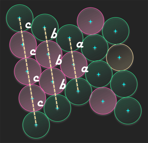
Image 22 – First method for intermediate points definitions

Second method:
• We trace the segments that connect the centers of adjacent circles. (segments BC and AC in Fig 23)
• We define the median planes normal to the segments
• (Plans  'and '' in fig 23)
• We define the lines of intersection before any other median planes
• We define the points of intersection between the straight lines and the surface (point D of Figure 23)
• We proceed in an iterative manner with the definition of all the other points.

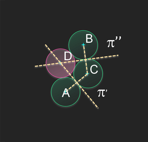
Image 23 – Generation of an equidistant point

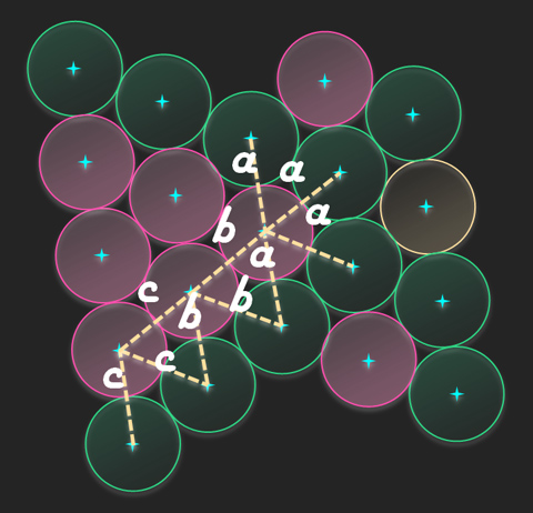
Image 24 - Second method for intermediate points definitions

The second system for the generation of intermediate points is currently used in the final version of the tool presented in this paper: however this strategy in some cases, does not guarantee an acceptable result for the generation.
In particular, if the adjacent circumferences tend to align, the intermediate circumference will tend to move away from the other in an excessive way, while keeping the condition of equidistance. Currently the tool does not apply any correction to this problem even with a new algorithm more effective and that is still under study.

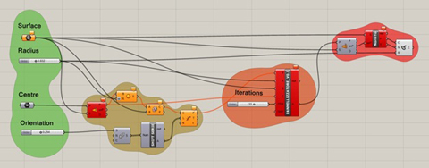
Image 25 – Paneling tool Grasshopper Scheme

Specifically, the tool was built using Visual Basic and Grasshopper.
More details can be found in the appendix to the contribution.
• To start to use the tool you need to set some input:
• Set the surface that you want to convert in a faceted tile,
• Set the radius of the circles, which is also the size of individual panels that form the tiling,
• Set a starting point of the definition,
• Set the orientation of the tiling,
• Set the number of iterations that must run the script (simply put the number of rings that make up the hexagonal mesh).
The output of the tool is a mesh of points which are approximately equidistant, usable for producing a paneling formed of highly repetitive elements.

Conclusions

At this point it’s important to consider the following aspects:
The tool is not perfect and it will require a second phase of development to improve the output. The most obvious problem refers to the outlying areas; the tool is not currently able to manage correctly and automatically the paneling near the border edges and it must be defined manually by a trick: expanding the edges of the surface so that the tool manages the original border areas as internal areas. The process is not automatic and it’s currently the only method that seems to work well, but still has some limitations: first a freeform UV surface can be extended beyond the edges in infinite ways. The manual procedure used is based on the extension of the curves U and V segments with tangents on both ends, but this does not mean that the extended surface is tangent to the original one. It really does not matter for our purpose: the border edges need to be extended only for the right positioning of the pattern points. Achieving this would be sufficient to make the tool more efficient and easier to use.
A second aspect that needs to be improved is the management of the tolerances of the paneling and the practical application in the construction phase.
In practice, the tool operates on the surface, creating a pattern where the individual units are not equal, but differ by a tolerance which varies in relation to the degree and type of curvature of the surface. The image 26 shows the same surface used previously with a false color representation in which colors represent the differences between the areas of each triangular panels.

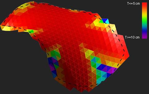
Image 26: the output surface in false color. The dotted line represents the original border.

The result is satisfactory: the output geometry contains 727 triangular panels, the majority are red (85% approximately), in other words the difference between areas tends to zero, only a very small percentage has an intermediate color (orange, yellow and green – 12%) and only a small amount in the outlying areas of panels are blue / purple (only 3%).
Moreover, the geometry requires cutting over the dotted black line, which represents the original edge of the surface (image 26), so the outlying areas must be redefined manually. Finally, we could use a single type of panel to cover all the red area: this means that we have a variable gap between each panels, but this will be easy to manage during installation phases (in this report we don’t enter into construction and installation themes): in a second phase of this job we could be taken into account the possibility of collaboration with façade construction companies and steelwork manufacturer to test the validity of the tool.

<a name="video01">Tolerances</a>

<a name="video02">Orientation</a>

<a name="video03">Eccentricity</a>